Superstructure Function Documentation

Author:

Christopher Laliwala, Oluwamayowa O. Amusat, Ana I. Torres

Date:

October 2025

Overview

This function employs superstructure optimization to identify optimal processing pathways for recovering materials from end-of-life products. The framework assumes discrete operations for first-stage disassembly and continuous operations for subsequent processing stages. Applications are demonstrated in [EVLaliwala2024] and [HDDLaliwala2024]. Users can optionally consider byproduct valorization and environmental impacts in their pathway selection.

Building Superstructure Model

The build_model() function constructs a Pyomo superstructure optimization model that identifies optimal processing pathways for recovering materials from end-of-life products. The function performs validation on all inputs, builds the mathematical model with appropriate variables and constraints, and returns a ConcreteModel ready for optimization.

Function Arguments

The arguments that must be passed to build the superstructure model are shown below:

Table 5 Arguments for the build_model function

Argument	Type	Description
Objective Function
obj_func	ObjectiveFunctionChoice	Choice of objective function. Options are ObjectiveFunctionChoice.NET_PRESENT_VALUE or ObjectiveFunctionChoice.COST_OF_RECOVERY.
Plant Lifetime Parameters
plant_start	int	The year that plant construction begins.
plant_lifetime	int	The total lifetime of the plant, including plant construction. Must be at least three years.
Feed Parameters
available_feed	dict	Total feedstock available (number of EOL products) for recycling each year.
collection_rate	float	Collection rate for how much available feed is processed by the plant each year.
tracked_comps	list	List of tracked components.
prod_comp_mass	dict	Mass of tracked components per EOL product (kg / EOL product).
Superstructure Formulation Parameters
num_stages	int	Number of total stages.
options_in_stage	dict	Number of options in each stage.
option_outlets	dict	Set of options k’ in stage j+1 connected to option k in stage j.
option_efficiencies	dict	Tracked component retention efficiency for each option.
Operating Parameters
profit	dict	Profit per unit of product in terms of tracked components ($/kg tracked component).
opt_var_oc_params	dict	Variable operating cost parameters for options that are continuous. Variable operating costs assumed to be proportional to the feed entering the option.
operators_per_discrete_unit	dict	Number of operators needed per discrete unit for options that utilize discrete units.
yearly_cost_per_unit	dict	Yearly operating costs per unit ($/year) for options which utilize discrete units.
capital_cost_per_unit	dict	Cost per unit ($) for options which utilize discrete units.
processing_rate	dict	Processing rate per unit for options that utilize discrete units. In terms of end-of-life products disassembled per year per unit (number of EOL products / year).
num_operators	dict	Number of operators needed for each continuous option.
labor_rate	float	Yearly wage per operator ($ / year).
Discretized Costing Parameters
discretized_purchased_equipment_cost	dict	Discretized cost by flows entering for each continuous option ($/kg).
Environmental Impacts Parameters
consider_environmental_impacts	bool	Choice of whether or not to consider environmental impacts.
options_environmental_impacts	dict	Environmental impacts matrix. Unit chosen indicator per unit of incoming flowrate.
epsilon	float	Epsilon factor for generating the Pareto front.
Byproduct Valorization Parameters
consider_byproduct_valorization	bool	Decide whether or not to consider the valorization of byproducts.
byproduct_values	dict	Byproducts considered, and their value ($/kg).
byproduct_opt_conversions	dict	Conversion factors for each byproduct for each option.

If NPV maximization is chosen, a mixed-integer linear programming model is constructed (MILP), if COR minimization is chosen, a mixed-integer quadratically constrained programming model is constructed (MIQCP). It is recommended that the user install Gurobi, as this solver can deal with both formulations, and also can deal with the SOS2 constraints that are generated for the piecewise-linear constraints.

Default Costing Parameters

The following table shows the default costing parameters used in the superstructure model. These values are based on NETL’s Quality Guidelines for Energy System Studies (QGESS) [Theis2021] and economic assumptions from Keim et al. (2019) [Keim2019]. All parameters are mutable and can be modified by the user after model creation.

Table 6 Default Costing Parameters

Parameter	Description	Default Value
lang_factor	Lang factor for calculating total plant cost from equipment costs.	2.97
i_operating_expense_escalation	Operating expenses escalation rate.	0.03 (3%)
i_capital_escalation	Capital expenses escalation rate.	0.036 (3.6%)
discount_factor	Discount factor for calculating the net present value. The after-tax weighted average cost of capital (ATWACC) is used.	0.0577 (5.77%)
financing_factor	Factor for calculating financing costs from total plant cost.	0.027 (2.7%)
other_costs_factor	Factor for calculating ‘other costs’ as defined by QGESS from the total plant cost.	0.15 (15%)
m_and_sm_costing_factor	Factor for calculating Maintenance & Supply Materials as a percentage of total plant cost.	0.02 (2%)
sa_and_qa_qc_costing_factor	Factor for calculating Sample Analysis & Quality Assurance/Quality Control as a percentage of cost of labor.	0.1 (10%)
s_ip_r_and_d_costing_factor	Factor for calculating Sales, Intellectual Property, and Research & Development as a percentage of total profit.	0.01 (1%)
a_and_sl_costing_factor	Factor for calculating Administrative & Supporting Labor as a percentage of cost of labor.	0.2 (20%)
fb_costing_factor	Factor for calculating Fringe Benefits as a percentage of cost of labor.	0.25 (25%)
pt_and_i_costing_factor	Factor for calculating Property Taxes & Insurance as a percentage of total plant cost.	0.01 (1%)
total_overnight_capital_fraction_expended	Fraction of total overnight capital expended in each year. 10% in year 1, 60% in year 2, and 30% in year 3.	Year 1: 0.1, Year 2: 0.6, Year 3: 0.3
plant_overhead_factor	Factor for calculating plant overhead as a percentage of total operating costs each year.	0.2 (20%)

Viewing Results

After building and solving the superstructure model, results can be reported to the console using the reporting functions in the prommis.superstructure.report_superstructure_results module. These functions provide detailed information about the optimal pathway selected, economic metrics, and environmental impacts.

The following reporting functions are available:

• report_optimal_pathway: Displays the selected processing options for each stage

• report_economics: Shows NPV, CAPEX, OPEX, and revenue breakdown

• report_material_flows: Reports component flows through the superstructure

• report_superstructure_environmental_impacts: Reports yearly and total environmental impacts generated by the process

Example usage:

from prommis.superstructure.report_superstructure_results import report_optimal_pathway

# After solving the model
report_optimal_pathway(model, results)

For detailed documentation of all reporting functions, see the Class Documentation section below.

Model Formulation

Mass Balance Equations

The superstructure is modeled as a network where the arrows represent flows and the boxes, or ‘nodes’, represent potential processing options (technologies). As depicted, these technologies are organized in stages.

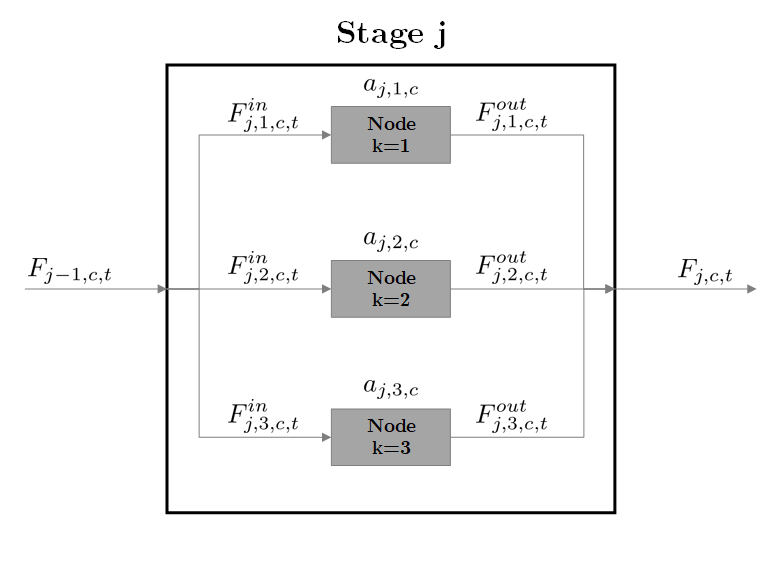
Fig. 3 Generic Mass Balance Diagram

Fig. 3 illustrates the mass balances for a generic stage \(j\). In this diagram, \(F_{j-1,c,t}\) is the upstream flow of component \(c\) coming from the previous stage \(j-1\) in year \(t\). \(F^{in}_{j,k,c,t}\) represents the inlet stream of component \(c\) entering node \(k\) in stage \(j\) at time \(t\). The sum of the inlet streams \(F^{in}_{j,k,c,t}\) is equal to the upstream flow, \(F_{j-1,c,t}\), as depicted in (1):

(1)\[F_{j-1,c,t} = \sum_{k \in K(j)} F^{in}_{j,k,c,t} \qquad \forall j \in J \setminus {j=1}, c \in C, t \in T\]

However, for the first stage, \(j=1\), the number of EOL products the plant processes in year \(t\) is represented by \(P^{entering}_{prod,t}\). Thus, the sum of the inlet streams \(F^{in}_{j,k,c,t}\) in the initial stage is equal to the flow of EOL product entering the plant. This is depicted in (2):

(2)\[P^{entering}_{prod,t} \cdot X_{prod,c,t} = \sum_{k \in K(j)} F^{in}_{j,k,c,t} \qquad j = 1, \quad \forall c \in C, t \in T\]

where \(X_{prod,c,t}\) is the amount of component \(c\) per EOL product in year \(t\).

Referring back to Fig. 3, \(F^{out}_{j,k,c,t}\) is the outlet stream of component \(c\) exiting node \(k\) in stage \(j\) at time \(t\) and is related to the inlet \(F^{in}_{j,k,c,t}\) by the efficiency parameter \(a_{j,k,c}\), as shown in (3):

(3)\[F^{in}_{j,k,c,t} \cdot a_{j,k,c} = F^{out}_{j,k,c,t} \qquad \forall j \in J, k \in K(j), c \in C, t \in T\]

where the efficiency parameter \(a_{j,k,c}\) represents the percentage of component \(c\) that is retained in node \(k\) in stage \(j\), and thus varies from 0 to 1.

Finally, the variable \(F_{j,c,t}\) represents the flow of component \(c\) exiting stage \(j\) at time \(t\), and is the sum of the outlet streams \(F^{out}_{j,k,c,t}\), as shown in (4).

(4)\[\sum_{k \in K(j)} F^{out}_{j,k,c,t} = F_{j,c,t} \qquad \forall j \in J \setminus {j=j_{final}}, c \in C, t \in T\]

Logical Constraints

To ensure that only one optimal pathway is chosen, logical constraints are formulated. We define the binary variables \(y_{j,k}\) for each node, which indicates whether node \(k\) in stage \(j\) is selected. Only one node per stage may be chosen ((5)). It is worth noting here that all stages include a blank node that allows the stage to be bypassed.

(5)\[\sum_{k \in K(j)} y_{j,k} = 1 \qquad \forall j \in J\]

Additionally, not all nodes are connected. Therefore, if a node in stage \(j \neq j_{final}\) is selected, a connected node must be chosen in the next stage. This is implemented in (6),

(6)\[\sum_{k' \in K(j,k)} y_{j+1,k'} \geq y_{j,k} \qquad\forall j \in J \setminus {j=4}\]

where \(k'\) is an alias for \(k\), and \(K(j,k)\) is the set of nodes in stage \(j+1\) that are connected to the node \(k\) in stage \(j\).

Finally, Big-M constraints are formulated to ensure that nodes that are not chosen have no flow through them ((7) and (8)).

(7)\[0 \leq F^{in}_{j,k,c,t} \leq y_{j,k} \cdot M_{j,k,c,t} \qquad \forall j \in J, k \in K(j), c \in C, t \in T\]

(8)\[0 \leq F^{out}_{j,k,c,t} \leq y_{j,k} \cdot M_{j,k,c,t} \qquad \forall j \in J, k \in K(j), c \in C, t \in T\]

Where \(M_{j,k,c,t}\) and \(M^{out}_{j,k,c,t}\) represent the upper bound of the flowrate.

Cost Equations

Capital Expenses

For the capital expenses, the methodology presented in NETL’s Quality Guidelines for Energy System Studies (QGESS) [Theis2021] is followed. However, since the methodology was developed for power plants, modifications to match the economic assumptions in Keim et al. (2019) [Keim2019] are made. It is important to note that all costing parameters (i.e. Lang Factor, financing, etc.) are all mutable parameters that can be changed by the user from their default values. Others, such as the product price \(Price_c\), must be provided by the user.

The capital cost levels from QGESS up until the Total Overnight Cost (\(TOC\)) are shown in Table 7. To calculate the \(TOC\), the total cost of purchased equipment is first calculated for each process node in the superstructure. Piecewise linear approximations are used for scaling equipment costs as functions of equipment size for all stages except disassembly, where discrete values are required. Next, the Total Plant Cost (\(TPC\)) is calculated by multiplying the updated total cost of purchased equipment by a Lang Factor (\(LF\)) [Keim2019] for each process node in all stages besides the disassembly stages and then summing them. For nodes in the disassembly stage, no Lang Factor is used. Thus, the TPC is computed as:

(9)\[TPC = LF \cdot \sum_{j \in J \setminus j=1} \sum_{k \in K(j)} C_{P,j,k} + \sum_{k \in K(j=1)} C_{P,j=1,k}\]

where \(C_{P,j,k}\) is the total cost of purchased equipment for node \(k\) in stage \(j\).

The \(TOC\) is calculated by (10):

(10)\[TOC = TPC + financing + other \: costs\]

where \(financing\) and \(other \: costs\) are 2.7% and 15% of the TPC, respectively [Theis2021].

Table 7 QGESS capital cost levels: Bare Erected Cost (BEC), Engineering, Procurement, and Construction Cost (EPCC), Total Plant Cost (TPC), and the Total Overnight Capital (TOC) [Theis2021].

Capital Cost Level	Includes:
BEC	Process equipment, Supporting facilities, Direct and indirect labor
EPCC	BEC and EPC contractor services
TPC	EPCC and Process contingency and Project contingency
TOC	TPC and Financing costs and Other owner’s costs

Operating Expenses (OPEX)

Both fixed and variable costs are considered for operating expenses. The variable operating costs account for utilities, reagents, and waste disposal and are assumed to be linearly related to the size of the process:

\[OPEX^{Var}_{j,k,t} = A_{j,k} \cdot F^{in,total}_{j,k,t} + B_{j,k} \cdot y_{j,k}\]

where \(A_{j,k}\) and \(B_{j,k}\) are the linear parameters for option \(k\) in stage \(j\), and \(F^{in,total}_{j,k,t}\) is the total flow entering the option.

For fixed operating costs, the cost of labor, maintenance and supply materials, quality assurance/quality control (QA/QC), sales, IP, R&D, administration and supporting labor, and property taxes and insurance were considered. To calculate the cost of labor (\(COL\)), we adopt the methodology described in Ulrich et al. (2004) [Ulrich2004], which assigns a number of operators to the different units. Other fixed costs are summarized in Table 8. \(R_t\) is the revenue in year \(t\).

Table 8 Summary of fixed costs other than the cost of labor considered [Keim2019].

Category	Value
Maintenance and Supply Materials (M&SM)	\(0.02 \cdot TPC\)
Sample Analysis & QA/QC (SA&QA/QC)	\(0.1 \cdot COL\)
Sales, IP, and R&D Costs (S,IP,R&D) in year \(t\)	\(0.01 \cdot R_t\)
Administrative & Supporting Labor (A&SL)	\(0.2 \cdot COL\)
Fringe benefits (FB)	\(0.25 \cdot COL\)
Property Taxes & Insurance (PT&I)	\(0.01 \cdot TPC\)

Cost of Labor

To calculate the cost of labor, the user must provide the yearly wage per operator, and the number of operators needed for each option. It is assumed that the plant operates for 8000 hours per year [Seider2017]. For the hourly wage per worker, we refer the user to [BLS2024], and for estimating the number of workers needed per option we refer them to [Ulrich2004] (in this methodology, the number of workers needed is independent of equipment sizing).

Since [Ulrich2004] methodology allows for fractions of workers (since workers can be responsible for multiple parts of a process), the following methodology is followed to calculate the total number of workers needed as an integer. First, the number of workers needed \(workers_{j,k}\), in fractional form for all stages besides the disassembly stage can be calculated using:

(11)\[workers_{j,k} = W_{j,k} * y_{j,k} \qquad \forall j \in J \setminus j=1, k \in K(j)\]

For nodes in the disassembly stage, either workers are employed or discrete units are utilized. Thus, the number of workers needed is dependent on the number of workers employed/units utilized for disassembly. The calculation for the number of workers needed, in fractional form, for all nodes in the disassembly stage is shown in (12):

(12)\[workers_{j,k} = W^{dis}_{j,k} * \sum_{i=0}^{max \: dis_{j,k}} i * y^{dis \: units}_{j,k,i} \qquad \forall j = 1, k \in K(j=1)\]

Where \(W^{dis}_{j,k}\) is the number of workers needed per disassembly unit/employee. \(y^{dis \: units}_{j,k,i}\) is a binary variable representing how many workers \(i\) are chosen for node \(k\) in the disassembly stage \(j_{dis}\), and \(max \: dis_{j,k}\) is a parameter representing the maximum number of units/workers for node k in the disassembly stage \(j_{dis}\) that could be utilized/employed.

For the disassembly nodes that employ workers instead of machinery, \(W_{j=1,k}\) is equal to one, as the number of workers needed is equal to the number employed for disassembly. To calculate the total number of workers employed as a whole number, (13) is utilized:

(13)\[\sum_{j \in J} \sum_{k \in K(j)} workers_{j,k} \leq \sum_{i=0}^{max \: workers} i * y^{workers}_i\]

Where \(y^{workers}_{i}\) is a binary variable representing how many total workers \(i\) are employed in the plant, and \(max \: workers\) is a parameter representing the maximum number of workers that can be employed.

To ensure only a single number of workers is employed, (14) is formulated:

(14)\[\sum_{i=0}^{max \: workers} y^{workers}_i = 1\]

Finally, the cost of labor, \(COL\), is calculated using (15):

(15)\[COL = wage * \sum_{i=0}^{max \: workers} i * y^{workers}_{i}\]

Where \(wage\) is the yearly wage per worker.

Revenues

The revenue in a given year \(t\) is calculated by multiplying the flow of each product leaving the final stage by its corresponding price, \(Price_c\) as shown in (16) [Keim2019].

(16)\[R_t = \sum_{k \in K(j=j_{final})} \sum_{c \in C} F^{out}_{j=j_{final},k,c,t} \cdot Price_{c} \qquad \forall t \in T\]

Objective Functions

Two objectives are available for users: maximizing the net present value (NPV), and minimizing the cost of recovery (COR), which estimates the selling price at which the NPV is zero.

Net Present Value

The NPV is given by:

(17)\[NPV = \sum_{t \in T} \frac{CF_t}{(1 + IR)^t}\]

Where \(CF_t\) is the cash flow in year \(t\), and \(IR\) is the interest rate. The cash flow was calculated using the methodology discussed in Seider et al. (2017) [Seider2017]. We modify the methodology to account for the assumptions for capital expenditure (\(TOC^{exp}_t\)), capital escalation (\(i^{esc,CAPEX}\)), and revenue and operating costs escalation (\(i^{esc,sales,OPEX}\)) [Keim2019]. The modified equation is shown in (18).

(18)\[CF_t = (R_t - OPEX_t) \cdot (1 + i^{esc,sales,OPEX})^{t - t_{prod \: start}} - TOC^{exp}_t \cdot (1 + i^{esc,CAPEX})^{t - t_{start}} \qquad \forall t \in T\]

where \(t_{start}\) is the year when the plant begins construction, \(t_{prod \: start}\) is the year when the plant begins production, and \(R_t\) and \(OPEX_t\) are the revenue and operating expenses in year \(t\), respectively. It was assumed that the capital costs would be spread over the first three years, with the expenditure being 10% in the first year, 60% in the second year, and 30% in the third year [Keim2019].

The NPV maximization problem is a mixed-integer linear optimization (MILP) problem.

Cost of Recovery

The COR is defined as the price of the product ($/kg) required for the NPV to break even. To introduce COR in the optimization problem, we modify the revenue expression ((16)),

(19)\[R_t = COR \cdot \sum_{k \in K(j=5)} \sum_{c \in C} F^{out}_{j=5,k,c,t} \qquad \forall t \in T\]

convert the NPV equation in (17) into a constraint, and set it to zero.

(20)\[NPV = \sum_{t \in T} \frac{CF_t}{(1 + IR)^t} = 0\]

(19) is non-linear, making the COR minimization a mixed-integer non-linear optimization (MINLP) problem.

Disassembly Stage

Since the disassembly stage utilizes discrete units, calculation of CAPEX and OPEX is different. First, the number of units utilized, or workers employed (depending on which option is chosen), is calculated such that the flow of incoming EOL products entering the plant can be disassembled without hold-up, as depicted in (21):

(21)\[P^{entering}_{prod,t} \leq Dis \: Rate_{j,k} * \sum_{k \in K} \sum_{i=0}^{i=max \: dis_{j,k}} i * y^{dis \: units}_{j,k,i} \qquad \forall j=1, k \in K(j=1), t \in T\]

Where \(Dis \: Rate_{j,k}\) is a parameter representing the rate of disassembly of the EOL product per unit/worker for node \(k\) in the disassembly stage \(j=1\) and must be provided by the user, \(y^{dis \: units}_{j,k,i}\) is a binary variable representing how many workers, \(i\), are chosen for node \(k\) in the disassembly stage \(j=1\), and \(max \: dis_{j,k}\) is a parameter representing the maximum number of units/workers for node \(k\) in the disassembly stage \(j=1\) that could be utilized/employed.

To ensure only a single number of units/workers is utilized/employed, (22) is formulated:

(22)\[\sum_{i=0}^{max \: dis_{j,k}} y^{dis \: units}_{j,k,i} = 1 \qquad \forall j = 1, k \in K(j=1)\]

Finally, to ensure no workers are utilized/employed if a disassembly node is not chosen, (23) is formulated:

(23)\[y_{j,k} \geq 1 - y^{dis \: units}_{j,k,i=0} \qquad j=1, k \in K(j=1)\]

CAPEX

For the nodes that employ workers, the CAPEX is zero. For the nodes that utilize discrete units, (24) is formulated:

(24)\[C_{P,j,k} = CU_{j,k} * \sum_{i=0}^{max \: dis_{j,k}} y^{dis \: units}_{j,k,i} * i \qquad \forall j=1, k \in K(j=1)\]

Where \(CU_{j,k}\) is a parameter representing the cost per unit for node \(k\) in the disassembly stage \(j=1\). The cost per unit for the disassembly nodes utilizing equipment for disassembly must be provided by the user.

Variable operating costs

To calculate the variable operating costs, \(OC^{var}_{j,k}\) for all nodes in the disassembly stage, (25) is utilized:

(25)\[OC^{var}_{j,k} = YCU_{j,k} * \sum_{i=0}^{max \: dis_{j,k}} y^{dis \: units}_{j,k,i} * i \qquad \forall j = 1, k \in K(j=1)\]

Where \(YCU_{j,k}\) is the yearly cost per unit for node \(k\) in stage \(j\). These values must be provided by the user.

Consideration of Byproduct Valorization

An additional capability of this function is for users to consider the valorization of byproducts into the overall economics of the process. If the user opts to include this, then a dict containing the byproducts considered and their value ($/kg) must be passed, along with a dict containing the conversion factors of the incoming total flowrate entering for each byproduct produced by each option.

The total amount of each byproduct produced each year is calculated:

\[F_{b,t} = \sum_{opt \in b(opt)} F_{opt,t}^{in, total} \cdot \alpha_{opt,b} \quad \forall b \in BP, t \in T\]

where \(F_{b,t}\) is the amount of byproduct \(b\) produced in year \(t\), \(F_{opt,t}^{in, total}\) is the total flow entering the option, \(\alpha_{opt,b}\) is the conversion factor for producing byproduct \(b\) in option \(opt\), \(b(opt)\) is the set of options that produce byproduct \(b\), and \(BP\) is the set of all byproducts.

The yearly profit from byproducts is calculated:

\[Byprod. \: Profit_t = \sum_{b \in BP} F_{b,t} \cdot Value_{b} \quad t \in T\]

where \(Value_b\) is the value of byproduct \(b\) in $/kg.

When byproduct valorization is considered, the calculation of the revenue is modified differently depending on which objective function is chosen. If the NPV is chosen, the revenue is calculated as:

\[R_t = Byprod. \: Profit_t + \sum_{k \in K(j=j_{final})} \sum_{c \in C} F^{out}_{j=j_{final},k,c,t} \cdot Price_{c} \quad \forall t \in T\]

and if the COR is chosen as the objective the revenue is calculated as:

\[R_t = Byprod. \: Profit_t + COR \cdot \sum_{k \in K(j=5)} \sum_{c \in C} F^{out}_{j=5,k,c,t} \quad \forall t \in T\]

Consideration of Environmental Impacts

The user also has the ability to consider environmental impacts of the potential processes. The choice of which environmental impacts is left up to the user. Typically, midpoint indicators are utilized to quantify environmental impacts. A common midpoint indicator tool for quantifying environmental impacts is the EPA’s Tool for the Reduction and Assessment of Chemical and Other Environmental Impacts (TRACI) [TRACI].

The total environmental impacts generated can be calculated by summing the impacts generated by each option over the lifetime of the plant:

\[EI = \sum_{t \in T} \sum_{opt \in OPTS} \theta_{opt} \cdot F^{in,total}_{opt,t}\]

where \(EI\) is the environmental impact chosen by the user, \(OPTS\) is the set of all options in the superstructure, and \(\theta_{opt}\) is a parameter for the amount of emissions generated by option \(opt\) per incoming feed entering and must be provided by the user, and \(F^{in,total}_{opt,t}\) is the flowrate entering option \(opt\) in year \(t\).

Consideration of environmental impacts leads to the formation of a multi-criteria optimization problem. This function utilizes the \(\epsilon\)-constraint method. By calling the function for varying values of \(\epsilon\), the user can construct the Pareto front.

Class Documentation

ObjectiveFunctionChoice

class prommis.superstructure.objective_function_enums.ObjectiveFunctionChoice(value, names=None, *, module=None, qualname=None, type=None, start=1, boundary=None)

Bases: Enum

Enum of supported objective functions

COST_OF_RECOVERY = 2

NET_PRESENT_VALUE = 1

Superstructure Function

Superstructure Code

Author: Chris Laliwala

class prommis.superstructure.superstructure_function.SuperstructureScaler(**kwargs)

Bases: CustomScalerBase

zero_tolerance

Value at which a variable will be considered equal to zero for scaling.

max_variable_scaling_factor

Maximum value for variable scaling factors.

min_variable_scaling_factor

Minimum value for variable scaling factors.

max_constraint_scaling_factor

Maximum value for constraint scaling factors.

min_constraint_scaling_factor

Minimum value for constraint scaling factors.

max_expression_scaling_hint

Maximum value for expression scaling hints.

min_expression_scaling_hint

Minimum value for constraint scaling hints.

overwrite

Whether to overwrite existing scaling factors.

constraint_scaling_routine(model, overwrite: bool = False, submodel_scalers: dict = None)

Routine to apply scaling factors to constraints in model.

Derived classes must overload this method.

Parameters:

• model – model to be scaled

• overwrite – whether to overwrite existing scaling factors

• submodel_scalers – ComponentMap of Scalers to use for sub-models

Returns:

None

variable_scaling_routine(model, overwrite: bool = False, submodel_scalers: dict = None)

Routine to apply scaling factors to variables in model.

Derived classes must overload this method.

Parameters:

• model – model to be scaled

• overwrite – whether to overwrite existing scaling factors

• submodel_scalers – ComponentMap of Scalers to use for sub-models

Returns:

None

prommis.superstructure.superstructure_function.build_model(obj_func, plant_start, plant_lifetime, available_feed, collection_rate, tracked_comps, prod_comp_mass, num_stages, options_in_stage, option_outlets, option_efficiencies, profit, opt_var_oc_params, operators_per_discrete_unit, yearly_cost_per_unit, capital_cost_per_unit, processing_rate, num_operators, labor_rate, discretized_purchased_equipment_cost, consider_environmental_impacts, options_environmental_impacts, epsilon, consider_byproduct_valorization, byproduct_values, byproduct_opt_conversions)

This function builds a superstructure model based on specifications from the user.

Parameters:

• obj_func (ObjectiveFunctionChoice) – Choice of objective function. Options are ObjectiveFunctionChoice.NET_PRESENT_VALUE or ObjectiveFunctionChoice.COST_OF_RECOVERY.

• plant_start (int) – The year that plant construction begins.

• plant_lifetime (int) – The total lifetime of the plant, including plant construction. Must be at least three years.

• available_feed (dict) – Total feedstock available (number of EOL products) for recycling each year.

• collection_rate (float) – Collection rate for how much available feed is processed by the plant each year.

• tracked_comps (list) – List of tracked components.

• prod_comp_mass (dict) – Mass of tracked components per EOL product (kg / EOL product).

• num_stages (int) – Number of total stages.

• options_in_stage (dict) – Number of options in each stage.

• option_outlets (dict) – Set of options k’ in stage j+1 connected to option k in stage j.

• option_efficiencies (dict) – Tracked component retention efficiency for each option.

• profit (dict) – Profit per unit of product in terms of tracked components ($/kg tracked component).

• opt_var_oc_params (dict) – Variable operating cost parameters for options that are continuous. Variable operating costs are assumed to be proportional to the feed entering the option.

• operators_per_discrete_unit (dict) – Number of operators needed per discrete unit for options that utilize discrete units.

• yearly_cost_per_unit (dict) – Yearly operating costs per unit ($/year) for options which utilize discrete units.

• capital_cost_per_unit (dict) – Cost per unit ($) for options which utilize discrete units.

• processing_rate (dict) – Processing rate per unit for options that utilize discrete units. In terms of end-of-life products disassembled per year per unit (number of EOL products / year).

• num_operators (dict) – Number of operators needed for each continuous option.

• labor_rate (float) – Yearly wage per operator ($ / year).

• discretized_purchased_equipment_cost (dict) – Discretized cost by flows entering for each continuous option ($/kg).

• consider_environmental_impacts (bool) – Choice of whether or not to consider environmental impacts.

• options_environmental_impacts (dict) – Environmental impacts matrix. Unit chosen indicator per unit of incoming flowrate.

• epsilon (float) – Epsilon factor for generating the Pareto front.

• consider_byproduct_valorization (bool) – Decide whether or not to consider the valorization of byproducts.

• byproduct_values (dict) – Byproducts considered, and their value ($/kg).

• byproduct_opt_conversions (dict) – Conversion factors for each byproduct for each option.

Returns:

Pyomo superstructure model.

Return type:

ConcreteModel

prommis.superstructure.superstructure_function.define_custom_units()

This function defines custom units that are needed throughout the model.

Report Superstructure Results

Report Superstructure Results Code

Author: Chris Laliwala

prommis.superstructure.report_superstructure_results.report_superstructure_costing(m, results=None)

This function reports the costing results of the superstructure. This includes the objective function value, the yearly cash flows, revenues, capital expenses, and operating expenses. Relevant costing parameters are also reported.

Parameters:

• m – Pyomo model

• results – Solver results object

prommis.superstructure.report_superstructure_results.report_superstructure_environmental_impacts(m, results=None)

This function reports the yearly, and total environmental impacts produced by the process. The user must specify the superstructure model to track environmental impacts for this function to work.

Parameters:

• m – Pyomo model

• results – Solver results object

prommis.superstructure.report_superstructure_results.report_superstructure_results_overview(m, results=None)

This function reports an overview of the results of solving the superstructure. This includes the optimal pathway, the objective function value, and the total environmental impacts if the user chose to track them.

Parameters:

• m – Pyomo model

• results – Solver results object

prommis.superstructure.report_superstructure_results.report_superstructure_streams(m, results=None)

This function reports the yearly values of the flow variables within the model. This includes flows entering each stage (f), flows entering each option (f_in), and flows exiting each option (f_out). If byproduct valorization is considered, then the yearly flows of byproducts produced are also reported.

Parameters:

• m – Pyomo model

• results – Solver results object

References

[EVLaliwala2024]

Laliwala, Christopher and Ana Torres. “Recycling Rare Earth Elements from End-of-Life Electric and Hybrid Electric Vehicle Motors.” Computer Aided Chemical Engineering 53 (2024): 1309-1314.

[HDDLaliwala2024]

Laliwala, Chris and Ana I. Torres. “Design and Optimization of Processes for Recovering Rare Earth Elements from End-of-Life Hard Disk Drives.” Systems & Control Transactions 3 (2024): 496-503.

[Keim2019] (1,2,3,4,5,6,7)

Keim, Steven A. “Production of Salable Rare Earths Products from Coal and Coal Byproducts in the U.S. Using Advanced Separation Processes: Phase 1.” Technical report, Marshall Miller & Associates, Inc., 2019.

[Theis2021] (1,2,3,4)

Theis, Joel. “Cost Estimation Methodology for NETL Assessments of Power Plant Performance.” Technical report, National Energy Technology Laboratory, 2021.

[Ulrich2004] (1,2,3)

Ulrich, Gael D. and Palligarnai T. Vasudevan. Chemical Engineering Process Design and Economics: A Practical Guide. Durham: Process Publishing, 2004.

[BLS2024]

U.S. Bureau of Labor Statistics. “Occupational Employment and Wages, May 2023.” 2024. https://www.bls.gov/oes/current/oes518091.htm. Accessed: 2024-09-16.

[TRACI]

EPA. “Tool for Reduction and Assessment of Chemicals and Other Environmental Impacts (TRACI).” 2024. https://www.epa.gov/chemical-research/tool-reduction-and-assessment-chemicals-and-other-environmental-impacts-traci. Accessed: 2025-10-12.

[Seider2017] (1,2)

Seider, Warren D., Daniel R. Lewin, J.D. Seader, Soemantri Widagdo, Rafiqul Gani, and Ka Ming Ng. Product and Process Design Principles. Hoboken, NJ: Wiley, 2017.